Block-based Fast Differentiable IIR in PyTorch

I recently came across a presentation by Andres Ezequiel Viso from GPU Audio at ADC 2022, in which he talked about how they accelerate IIR filters on the GPU. The approach they use is to formulate the IIR filter as a state-space model (SSM) and augment the transition matrix so that each step processes multiple samples at once. The primary speedup stems from the fact that GPUs are very good at performing large matrix multiplications, and the SSM formulation enables us to leverage this capability.

Speeding up IIR filters while maintaining differentiability has always been my interest. The most recent method I worked on is from my recent submission to DAFx 25, where my co-author Ben proposed using parallel associative scan to speed up the recursion on the GPU. Nevertheless, since PyTorch does not have a built-in associative scan operator (in contrast to JAX), we must implement custom kernels for it, which is non-trivial. It also requires that the filter has distinct poles so that the state-space transition matrix is diagonalisable. The method that GPU Audio presented appears to be feasible solely using the PyTorch Python API and doesn’t have the restrictions I mentioned; thus, I decided to benchmark it and see how it performs.

Since it’s just a proof of concept, the filter I’m going to test is a time-invariant all-pole IIR filter, which is the minimal case of a recursive filter. This allows us to leverage some special optimisations that won’t work with time-varying general IIR filters, but that won’t affect the main idea I’m going to present here.

Naive implementation of an all-pole IIR filter

The difference equation of an \(M\)-th order all-pole IIR filter is given by:

Let’s implement this in PyTorch:

import torch
from torch import Tensor

@torch.jit.script
def naive_allpole(x: Tensor, a: Tensor) -> Tensor:
    """
    Naive all-pole filter implementation.
    
    Args:
        x (Tensor): Input signal.
        a (Tensor): All-pole coefficients.
        
    Returns:
        Tensor: Filtered output signal.
    """
    assert x.dim() == 2, "Input signal must be a 2D tensor (batch_size, signal_length)"
    assert a.dim() == 1, "All-pole coefficients must be a 1D tensor"

    # list to store output at each time step
    output = []
    # assume initial condition is zero
    zi = x.new_zeros(x.size(0), a.size(0))

    for xt in x.unbind(1):
        # use addmv for efficient matrix-vector multiplication
        yt = torch.addmv(xt, zi, a, alpha=-1.0)
        output.append(yt)

        # update the state for the next time step
        zi = torch.cat([yt.unsqueeze(1), zi[:, :-1]], dim=1)

    return torch.stack(output, dim=1)

In this implementation, I didn’t use any in-place operations for speedup since it would break the differentiability of the function. This naive implementation is not very efficient, as torch.addmv and torch.cat are called at each time step. Typically, the audio signal is hundreds of thousands of samples long, resulting in a significant amount of function call overhead. For details, please take a look at my tutorial on differentiable IIR filters at ISMIR 2023.

Notice that I used torch.jit.script to compile the function for some slight speedup. I tried the newer compilation feature torch.compile, but it didn’t work. The compilation hangs forever, I don’t know why… I never found torch.compile to be useful in my research projects, and torch.jit.* has proven to be way more reliable.

Let’s benchmark its speed on my Ubuntu with an Intel i7-7700K. We’ll use a batch size of 8, a signal length of 16384, and \(M=2\), which is a reasonable setting for audio processing.

from torch.utils.benchmark import Timer

batch_size = 8
signal_length = 16384
order = 2

def order2a(order: int) -> Tensor:
    a = torch.randn(order)
    # simple way to ensure stability
    a = a / a.abs().sum()
    return a

a = order2a(order)
x = torch.randn(batch_size, signal_length)

naive_allpole_t = Timer(
    stmt="naive_allpole(x, a)",
    globals={"naive_allpole": naive_allpole, "x": x, "a": a},
    label="naive_allpole",
    description="Naive All-Pole Filter",
    num_threads=4,
)
naive_allpole_t.blocked_autorange(min_run_time=1.0)

<torch.utils.benchmark.utils.common.Measurement object at 0x7f5b4423b260>
naive_allpole
Naive All-Pole Filter
  Median: 168.93 ms
  IQR:    0.54 ms (168.57 to 169.11)
  6 measurements, 1 runs per measurement, 4 threads

168.93 ms is relatively slow, but it is expected.

State-space model formulation

Before we proceed to showing the sample unrolling trick, let’s first introduce the state-space model (SSM) formulation of the all-pole IIR filter. The model is similar to the one used in my previous blogpost on TDF-II filter:

Here, I simplified the original SSM by omitting the direct path, as it can be derived from the state vector (for the all-pole filter only). Below is the PyTorch implementation of it:

@torch.jit.script
def a2companion(a: Tensor) -> Tensor:
    """
    Convert all-pole coefficients to a companion matrix.

    Args:
        a (Tensor): All-pole coefficients.

    Returns:
        Tensor: Companion matrix.
    """
    assert a.dim() == 1, "All-pole coefficients must be a 1D tensor"
    order = a.size(0)
    c = torch.diag(a.new_ones(order - 1), -1)
    c[0, :] = -a
    return c

@torch.jit.script
def state_space_allpole(x: Tensor, a: Tensor) -> Tensor:
    """
    State-space implementation of all-pole filtering.

    Args:
        x (Tensor): Input signal.
        a (Tensor): All-pole coefficients.

    Returns:
        Tensor: Filtered output signal.
    """
    assert x.dim() == 2, "Input signal must be a 2D tensor (batch_size, signal_length)"
    assert a.dim() == 1, "All-pole coefficients must be a 1D tensor"

    c = a2companion(a).T

    output = []
    # assume initial condition is zero
    h = x.new_zeros(x.size(0), c.size(0))

    # B * x
    x = torch.cat(
        [x.unsqueeze(-1), x.new_zeros(x.size(0), x.size(1), c.size(0) - 1)], dim=2
    )

    for xt in x.unbind(1):
        h = torch.addmm(xt, h, c)
        # B^T @ h
        output.append(h[:, 0])
    return torch.stack(output, dim=1)

a2companion converts the all-pole coefficients to a companion matrix, which is \(\mathbf{A}\) in the SSM formulation.

Before we benchmark the speed of this implementation, let’s predict how fast it will be. Intuitively, since the complexity of vector-dot product is \(O(M)\) and matrix-vector multiplication is \(O(M^2)\), the SSM implementation uses more computational resources, so it should be slower than the naive implementation. Let’s benchmark its speed:

state_space_allpole_t = Timer(
    stmt="state_space_allpole(x, a)",
    globals={"state_space_allpole": state_space_allpole, "x": x, "a": a},
    label="state_space_allpole",
    description="State-Space All-Pole Filter",
    num_threads=4,
)
state_space_allpole_t.blocked_autorange(min_run_time=1.0)

<torch.utils.benchmark.utils.common.Measurement object at 0x7f5a02eaf4a0>
state_space_allpole
State-Space All-Pole Filter
  Median: 118.41 ms
  IQR:    1.17 ms (117.79 to 118.96)
  9 measurements, 1 runs per measurement, 4 threads

Interestingly, the SSM implementation is approximately 50 ms faster.

By using torch.profiler.profile, I found that, in the naive implementation, torch.cat for updating the last M outputs accounts for a significant portion of the total time (~20%). The actual computation, torch.addmv, takes only about 10% of the time. Regarding memory usage, the most memory-intensive operation is torch.addmv, which consumes approximately 512 Kb of memory. In contrast, the SSM implementation uses more memory (> 1 Mb) due to matrix multiplication, but roughly 38% of the time is spent on filtering since it no longer has to call torch.cat at each time step. The state vector (a.k.a the last M outputs) is automatically updated during the matrix multiplication.

Conclusion: Tensor concatenation (including torch.cat and torch.stack) is computationally expensive, and it is advisable to avoid it whenever possible.

Unrolling the SSM

Now we can apply the unrolling trick to the SSM implementation. The idea is to divide the input signal into blocks of size \(T\) and perform the recursion on these blocks instead of processing them sample-by-sample. Each recursion takes the last vector state \(\mathbf{h}[n-1]\) and predicts the next \(T\) states \([\mathbf{h}[n], \mathbf{h}[n+1], \ldots, \mathbf{h}[n+T-1]]^\top\) at once. To see how to calculate these states, let’s unroll the SSM recursion for \(T\) steps:

We can rewrite the above equation in matrix form as follows:

Notice that in the second line, I utilised the fact that \(\mathbf{B}\) has only one non-zero entry to simplify the matrix. (This is not possible if the filter is not strictly all-pole.) \(\mathbf{I}_{.1}\) denotes the first column of the identity matrix and so on.

Now, the number of autoregressive steps is reduced from \(T\) to \(\frac{N}{T}\) and the matrix multiplication is done in parallel for every \(T\) samples. There are added costs for pre-computing the transition matrix \(\mathbf{M}\) and the input matrix \(\mathbf{V}\), though. However, as long as the extra cost is relatively small compared to the cost of \(T\) autoregressive steps, we should observe a speedup.

Here’s the PyTorch implementation of the unrolled SSM:

@torch.jit.script
def state_space_allpole_unrolled(
    x: Tensor, a: Tensor, unroll_factor: int = 1
) -> Tensor:
    """
    Unrolled state-space implementation of all-pole filtering.

    Args:
        x (Tensor): Input signal.
        a (Tensor): All-pole coefficients.
        unroll_factor (int): Factor by which to unroll the loop.

    Returns:
        Tensor: Filtered output signal.
    """
    if unroll_factor == 1:
        return state_space_allpole(x, a)
    elif unroll_factor < 1:
        raise ValueError("Unroll factor must be >= 1")

    assert x.dim() == 2, "Input signal must be a 2D tensor (batch_size, signal_length)"
    assert a.dim() == 1, "All-pole coefficients must be a 1D tensor"
    assert (
        x.size(1) % unroll_factor == 0
    ), "Signal length must be divisible by unroll factor"

    c = a2companion(a)

    # create an initial identity matrix
    initial = torch.eye(c.size(0), device=c.device, dtype=c.dtype)
    c_list = [initial]
    # TODO: use parallel scan to improve speed
    for _ in range(unroll_factor):
        c_list.append(c_list[-1] @ c)

    # c_list = [I c c^2 ... c^unroll_factor]
    M = torch.cat(c_list[1:], dim=0).T
    flatten_c_list = torch.cat(
        [c.new_zeros(c.size(0) * (unroll_factor - 1))]
        + [xx[:, 0] for xx in c_list[:-1]],
        dim=0,
    )
    V = flatten_c_list.unfold(0, c.size(0) * unroll_factor, c.size(0)).flip(0)

    # divide the input signal into blocks of size unroll_factor
    unrolled_x = x.unflatten(1, (-1, unroll_factor)) @ V

    output = []
    # assume initial condition is zero
    h = x.new_zeros(x.size(0), c.size(0))
    for xt in unrolled_x.unbind(1):
        h = torch.addmm(xt, h, M)
        # B^T @ h
        output.append(h[:, :: c.size(0)])
        h = h[
            :, -c.size(0) :
        ]  # take the last state vector as the initial condition for the next step
    return torch.cat(output, dim=1)

The unroll_factor parameter controls the number of samples to process in parallel. If it is set to 1, the function is the original SSM implementation.

Now let’s benchmark the speed of the unrolled SSM implementation. We’ll use unroll_factor=128 since I already tested that it is the optimal value :)

state_space_allpole_unrolled_t = Timer(
    stmt="state_space_allpole_unrolled(x, a, unroll_factor=unroll_factor)",
    globals={
        "state_space_allpole_unrolled": state_space_allpole_unrolled,
        "x": x,
        "a": a,
        "unroll_factor": 128,
    },
    label="state_space_allpole_unrolled",
    description="State-Space All-Pole Filter Unrolled",
    num_threads=4,
)
state_space_allpole_unrolled_t.blocked_autorange(min_run_time=1.0)

<torch.utils.benchmark.utils.common.Measurement object at 0x7f5a01d75160>
state_space_allpole_unrolled
State-Space All-Pole Filter Unrolled
  Median: 1.89 ms
  IQR:    0.08 ms (1.88 to 1.96)
  6 measurements, 100 runs per measurement, 4 threads

1.89 ms! What sorcery is this? That’s a whopping 60x speedup compared to the standard SSM implementation!

A closer look at the profiling results shows that in total, 38% of the time is spent on matrix multiplication and addition. The speedup comes with a cost of increased memory usage, requiring more than 2 MB for filtering. Not a significant cost for modern Hardwares.

For convenience, I ran the above benchmarks using the CPU, which has very limited parallelism compared to the GPU. Thus, the significant speedup we observe indicates that function call overhead is the major bottleneck for running recursions.

More comparison

Since \(T\) is an essential parameter for the unrolled SSM, I did some benchmarks to see how it affects the speed.

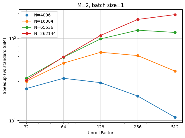
Varying sequence length

In this benchmark, I fixed the batch size to 8 and the order to 2, and varied the sequence length from 4096 to 262144. The results suggest that the best unroll factor increases as the sequence length increases, and it’s very likely to be \(\sqrt{N}\). Additionally, the longer the sequence length, the greater the speedup we achieve from the unrolled SSM.

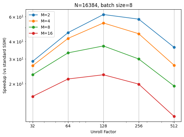
Varying filter order

To examine the impact of filter order on speed, I set the batch size to 8 and the sequence length to 16384, and then varied the filter order from 2 to 16. It appears that my hypothesis that the best factor is \(\sqrt{N}\) still holds, but the peak gradually shifts to the left as the order increases. Moreover, the speedup is less significant for higher orders, which is expected as the \(\mathbf{V}\) matrix becomes larger.

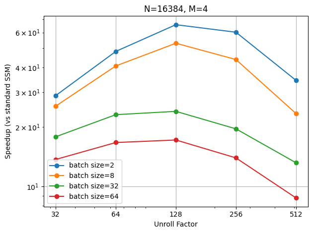
Varying batch size

The speedup is less as the batch size increases, which is expected. However, the peak of the best unroll factor also shifts slightly to the left as the batch size increases.

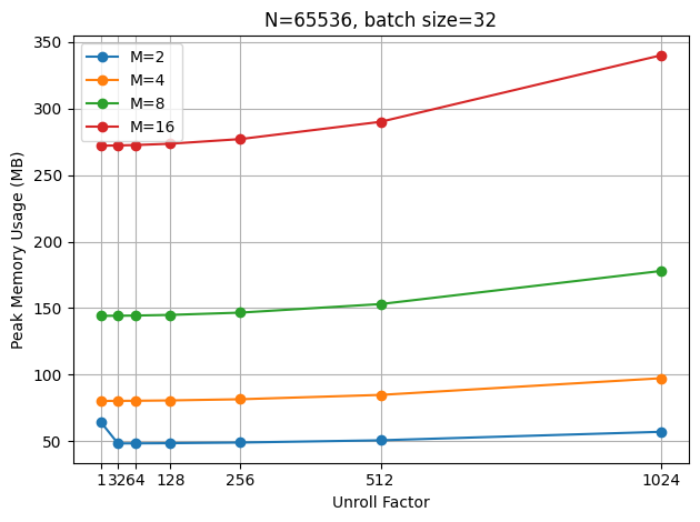
Memory usage

To observe how memory usage changes in a differentiable training context, I ran the unrolled SSM on a 5060 Ti, allowing me to use torch.cuda.max_memory_allocated() to measure memory usage. When batch size is 1, as expected, the memory usage grows quadratically with the unroll factor, due to the creation of the \(\mathbf{V}\) matrix.

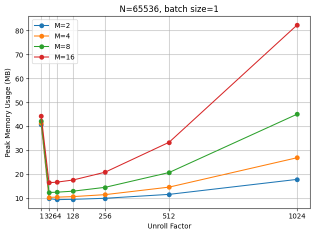
When using a larger batch size (32 in this case), this cost becomes less significant compared to the more memory used for the input signal.

Discussion

So far, we have seen that the unrolled SSM can achieve a significant speedup for IIR filtering in PyTorch. However, determining the best unrolling factor automatically is still unclear. From the benchmarks I did on an i7 CPU, it seems that the optimal \(T^*\) is \(\sqrt{N}\alpha\) and \(0 < \alpha \leq 1\) is given by a function of the filter order and batch size. Since I also observe similar behaviour on the GPU, it is likely that this hypothesis holds true for other hardware as well.

One thing I didn’t mention is numerical accuracy. If \(|\mathbf{A}|\) is very small, the precomputed exponentials \(\mathbf{A}^T \to \mathbf{0}\) which may not be accurately represented in floating point, especially in deep learning applications we use single precision a lot. This is less of a problem for the standard SSM, since at each time step, the input is mixed with the state vector, which could help cancel out the numerical errors.

The idea should apply when there are zeros in the filter. \(\mathbf{B}\) will not be a simple one-hot vector anymore so \(\mathbf{V}\) has to be a full \(MT\times MT\) square matrix. Time-varying filters will benefit less from the unrolling trick since \(\mathbf{V}\) will also be time-varying, and computing \(\frac{N}{T}\) such matrices in advance increases the cost.

Conclusion & Thoughts

In this post, I demonstrate that the unrolling trick can significantly accelerate differentiable IIR filtering in PyTorch. The extra memory cost is less of a problem for large batch sizes. Although the filter I tested is a simple all-pole filter, it’s trivial to extend the idea to general IIR filters.

This method might help address one of the issues for future TorchAudio, after the Meta developers announced their future plan for it. In the next major release, all the specialised kernels written in C++, including the lfilter I contributed years ago, will be removed from TorchAudio. The filter I presented here is written entirely in Python, and it could serve as a straightforward drop-in replacement for the current compiled lfilter implementation.

Notes

The complete code is available in the Jupyter notebook version of this post on Gist.